

3 The h1 Tool Suite through Examples
The h1 prover is the core of the h1 tool suite, and we
shall explain the tool suite by running h1 on several examples.
The h1 prover is invoked by calling h1 with a sequence of
flags, ended by a file name. The file name should contain a set of
clauses in TPTP clause format. Such files conventionally end with the
.p extension—but there is no obligation. Also, giving a
single dash - as file name forces h1 to read the input
clause set from standard input.
3.1 A Toy, Introductory Example
Examples are given in the distribution package. Here is a very small
one (file test1.p):
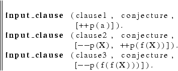
This contains three clauses. Each clause is introduced by the keyword
input_clause. The first argument,
clause1,
clause2, or
clause3 above, is the name of the clause.
Names are used in sundry ways, mainly for explanation and
documentation purposes. It is good practice to give each clause a
different name, but the tools of the h1 tool suite should work
even when several clauses have the same name.
The second argument can be the keyword
conjecture or
axiom; h1 just does not care: write
what you prefer here.
Finally, the third argument, enclosed between square brackets, is the
clause itself. It is a list of literals, separated by commas. Each
literal starts with a sign, ++ for positive
literals, -- for negative literals. The
clauses above are, in a more traditional notation:
| |
p(a) |
|
| |
¬ p (X) or p (f (X)) |
|
| |
¬ p (f (f (X))) |
| p (a) |
|
|
| p (f (X)) |
:- |
p (X) |
| false |
:- |
p (f (f (X))) |
Launch h1 on this file, test1.p, by typing
h1 test1.p
You will get the answer
*** Derived: clause3 ***
which means that a contradiction was found, using the clause named
clause3 in the last step. In other words, in the present
example, it says that a fact of the form p (f (f (t))), matching the
body of clause3, can be deduced from the definite clauses
(here, clause1 and clause2)
So far, so good, this is typically the least you could expect from a
theorem prover.
However, h1 also produced two more files, test1.log
and test1.model.pl. If you're curious, look at
test1.log, by running
less test1.log
Oh well, it is long, but it is not meant to be read by a human reader!
If you're perspicuous enough, you'll find some meaning buried inside
this. However, this is really meant as a log file, from which h1trace can extract a (mostly) readable proof
(Section 5), and which h1mc can use to get some
essential information it needs (Section 6).
3.2 The Dreadsbury Mansion Murder Mystery Example
Here is a more complicated example, due to Len Schubert. This is
problem 55 of [1986 (Pelletier)].
Someone in Dreadsbury Mansion killed Aunt Agatha. Agatha, the
butler, and Charles live in Dreadsbury Mansion, and are the only
ones to live there. A killer always hates, and is no richer than
his victim. Charles hates noone that Agatha hates. Agatha hates
everybody except the butler. The butler hates everyone not richer
than Aunt Agatha. The butler hates everyone whom Agatha hates.
Noone hates everyone. Who killed Agatha?
The problem is formalized in file butler-puzzle.p. The clauses
are as follows. First, “Agatha, the butler, and Charles live in
Dreadsbury Mansion, and are the only ones to live there.”:
|
|
agatha_in_mansion |
in_mansion (agatha) |
|
|
charles_in_mansion |
in_mansion (charles) |
|
|
butler_in_mansion |
in_mansion (butler) |
|
|
|
|
killer_hates_victim |
hates (X,Y) |
:- |
killed (X,Y) |
killer_no_richer |
not_richer (X,Y) |
:- |
killed (X,Y) |
|
|
|
charles_hates_noone_agatha_hates |
false |
:- |
hates (charles,X), hates (agatha,X) |
|
|
|
Agatha_hates_herself |
hates (agatha, agatha) |
|
|
Agatha_hates_charles |
hates (agatha, charles) |
|
|
|
|
butler_hates_everyone_not_richer_than_agatha |
hates (butler, X) |
:- |
not_richer (X, agatha) |
|
|
|
butler_hates_everybody_agatha_hates |
hates (butler, X) |
:- |
hates (agatha, X) |
|
|
|
noone_hates_everyone |
false |
:- |
hates (X,agatha), hates (X,butler), hates (X, charles) |
|
|
|
WHO_killed_agatha |
killed (WHO, agatha) |
|
cpp -P -DWHO=butler butler-puzzle.p | h1 -
You get the output:
*** Derived: noone_hates_everyone ***
In other words, the butler cannot have killed Agatha (contrarily to
proper conventions in popular whodunnit mysteries), because this would
contradict the fact that noone hates everyone.
More information can be gotten from the trace file h1out.log.
(Running h1 on file <file>.p produces a trace file
<file>.log. If no input file is given, as here, the trace file
is called h1out.log.) We shall explain how to use this trace
file in Section 5. For now, just run
h1trace h1out.log >dummy
and open the file dummy. You'll see that the first lines say:
. #false(noone_hates_everyone) [noone_hates_everyone].
using assumption #false(noone_hates_everyone) :-
hates(X1,charles), hates(X1,butler), hates(X1,agatha).
{X1=butler}
In other words, assuming the butler killed Agatha would involve that
the butler hates everyone, which is impossible. The rest of file dummy is a tree-like proof that indeed the butler hates everyone,
i.e., hates Agatha, Charles, and himself in this case.
So did Charles kill Agatha instead?
cpp -P -DWHO=charles butler-puzzle.p | h1 -
No, this would contradict the fact that Charles hates noone that
Agatha hates. In this case, Charles hates Agatha, and Agatha hates
herself, whence the contradiction.
*** Derived: charles_hates_noone_agatha_hates ***
There is only one possibility remaining: that Agatha killed herself.
cpp -P -DWHO=agatha butler-puzzle.p | h1 -
and indeed, h1 does not complain: assuming Agatha killed herself
leads to no contradiction. The file h1out.model.pl describes
the least model of this clause set.
This could have been found automatically by a simple sh script,
listing all possible murderers of Aunt Agatha.
for who in butler charles agatha
do
  if (cpp -P -DWHO=$who butler-puzzle.p | h1 - 2>&1\
                                        | grep -q Derived)
  then echo $who did not kill agatha.
  else echo $who may have killed agatha.
  fi
done
Since somebody killed Agatha, it must be herself.
butler did not kill agatha.
charles did not kill agatha.
agatha may have killed agatha.
The point of this example is that, first, the clauses are clearly not
(alternating tree) automata clauses; and second, that they are
H1 clauses. Check this by running h1 with the -check-h1 2 option:
cpp -P -DWHO=agatha butler-puzzle.p | h1 -check-h1 2 -
This makes h1 run as above, except it would have failed if any
of the input clauses where not in H1. By default, h1 runs as h1 -check-h1 0, which does not check anything, but
computes an approximation, see Section 3.4.
That the clauses of butler-puzzle.p are in the H1
class may seem surprising. After all, H1 clauses are
required to use only unary predicates, i.e., all predicate
letters P can only take one argument. This is certainly not the
case of the hates, killed, and
not_richer predicates above, which are all binary!
The trick here is that, when h1 sees an n-ary predicate P
(t1, …, tn) in its input, it converts it first to P (fP
(t1, …, tn)) for some fresh n-ary function symbol fP.
(Different occurrences of P correspond to the same symbol fP.)
This makes P unary, and does not change the semantics of clauses in
any essential way. Under the hood, h1 typically builds fP by
prepending a sharp sign # in front of the name of P,
guaranteeing that no clash occurs with any function symbol you may
have used. Don't count on it, though, as this may change in future
releases. Also, the h1 tools try to hide this kludge as much as
they can, and will happily parse and print n-ary predicate symbols.
We shall return to this example in Section 3.3.8.
3.3 Computing with Tree Automata
Assume that we wish to compute the intersection of the languages
L1 of all lists of even natural numbers, and L2 of all trees with binary nodes labeled with cons, and whose
leaves are either nil or natural numbers of the form 3n+2,
n in |N.
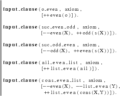
We have already seen what an automaton recognizing L1
looked like, see Figure 1. In TPTP format, this is
file listeven.p:
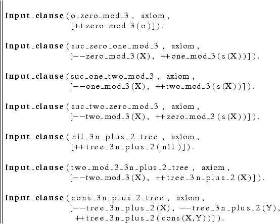
The language L2 is described by the predicate (final
state) tree_3n_plus_2. Look at file tree3plus2.p:
By the way, we can convert any automaton in TPTP format into Prolog
format by running h1 with the -no-trim option:
h1 -no-trim tree3plus2.p
Normally, h1's default is
to use the -trim option, which trims away all clauses that are obviously not needed for
deriving a contradiction. (See Section 4.1 for more
information on -trim and -no-trim.) In this case,
trimming would just eliminate all clauses! Since we are not looking
for a contradiction, we just run h1 without trimming, and get a
model in tree3plus2.model.pl:

In other words, h1 can be used to convert any set of H1 clauses into an equivalent alternating tree automaton by running
it
with the -no-trim option and looking into the generated model file, ending in .model.pl.
3.3.1 Visualizing Tree Automata
Before we compute the intersection of L1 and L2, let us visualize the automaton defining L2. This is
accomplished using pl2gastex, see Figure 2. For more information on pl2gastex, and how to read such pictures precisely, see
Section 13.
Figure 2:
Trees with leaves equal to
nil or to 3
n+2,
n in |N
3.3.2 Computing Intersections of Tree Automata
Now compute the intersection. Build a file, say
list_even_inter_tree3plus2.p, by concatenating the clauses from
listeven.p and from tree3plus2.p, and add the so-called
intersection clause
| q (X) |
:- |
list_even (X), tree_3n_plus_2 (X) |
tree_3n_plus_2. Just run the following
commands:
OUT=list_even_inter_tree3plus2
cat listeven.p tree3plus2.p >$OUT.p
echo "input_clause ($OUT, axiom, \
        [++q(X), --list_even(X),\
        --tree_3n_plus_2(X)])" >>$OUT.p
Because of the intersection
clause above, the resulting clause set is not an alternating tree
automaton as we have defined it. However, run h1 -no-trim on it:
h1 -no-trim list_even_inter_tree3plus2.p
and look at the generated alternating tree automaton. This is
obtained, as usual, in a file named
list_even_inter_tree3plus2.model.pl:
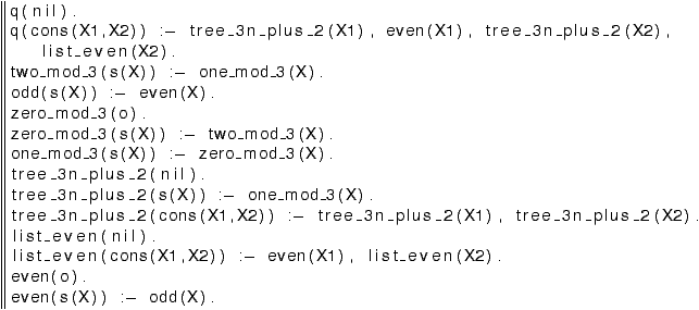
Graphically, this is the alternating tree automaton of
Figure 3.
Figure 3:
Trees with leaves equal to
nil or to 3
n+2, which are lists of even natural numbers at the same time
Note the presence of new nodes labeled ∧ in
Figure 3. They represent intersections of languages.
Indeed, there are two ways one can construct an element of
q. First, there is nil. Second, there are terms of the
form cons applied to two arguments X1 and X2, where X1 is
recognized both at tree_3n_plus_2
and at even, and X2 is recognized both at tree_3n_plus_2 and at
list_even.
The alternating tree automaton above recognizes (at q) the terms in
the intersection of L1 and L2. One should
observe that computing intersections of two languages by concatenating
the clause sets defining each and adding an intersection clause is
rather cavalier. It is only correct here because the two files
listeven.p and tree3plus2.p share no predicate symbol.
In general, one might allow shared predicate symbols, provided they
have the same semantics in each file. For example, it is legal for
the two files to both use the predicate
even provided it denotes the set of even
natural numbers in both. Otherwise, strange things may happen (an
over-approximation will be computed).
3.3.3 Checking Tree Automata for Emptiness, Testing Membership
It may not be completely obvious whether such an alternating tree
automaton is empty or not. (To say the least. The problem is
DEXPTIME-complete.) Let us see whether the intersection state
q is empty or not. In general, given a
satisfiable set S of Horn clauses (e.g., definite clauses, in
particular alternating tree automata clauses), the language of terms
recognized at state P in S is empty if and only if S plus the
clause false :- P (X) is satisfiable. Running:
(cat list_even_inter_tree3plus2.p;\
 echo "input_clause(q_is_not_empty, conjecture, [--q(X)]).")\
  | h1 -log-out - >list_even_inter_tree3plus2.log
yields *** Derived: q_is_not_empty ***
meaning that there are
indeed terms recognized at state q in the intersection.
We have kept a trace of the derivation in the log file
list\_even\_inter\_tree3plus2.log. We can then use h1trace to get a mostly readable proof of the fact that q is non-empty; in
particular, to have an example of a term recognized at q:
%-*-mode:outline;outline-regexp:"[0-9a-z.]+"-*-
. #false(q_is_not_empty).
  using assumption #false(q_is_not_empty) :- q(X1).
   {X1=nil}
1. q(nil).
    using assumption q(X1) :- tree_3n_plus_2(X1), list_even(X1).
     {X1=nil}
1.1. tree_3n_plus_2(nil) by assumption.
1.2. list_even(nil) by assumption.
In fact, the empty
list nil is recognized at q ({X1=nil} at line 4 above).
How to read such proofs will be explained in
Section 5.
Let us test membership of some ground term. Is the list cons (s (s
(o)), nil) consisting of just the natural number 2 in the
intersection? In general, given S as above, a ground term t is
recognized at state P if and only if S plus the clause false
:- P (t) is satisfiable.
(cat list_even_inter_tree3plus2.p;\
 echo "input_clause(q_rec_cons_2_nil, conjecture,\
         [--q(cons(s(s(o)),nil))]).")\
  | h1 -
yields
*** Derived: q_rec_cons_2_nil ***
So cons (s (s (o)), nil) is
in the intersection.
On the other hand, the list cons (s (s (s (s (o)))), nil) containing
just the natural number 4 is not in the intersection. Run
(cat list_even_inter_tree3plus2.p;\
 echo "input_clause(q_rec_cons_4_nil, conjecture,\
         [--q(cons(s(s(s(s(o)))),nil))]).")\
  | h1 -
and you'll get
(no message at all). Indeed,
cons (s (s (s (s (o)))), nil) is a list of even natural numbers, but
not a tree whose numeric leaves are of the form 3n+2, n in |N.
We can do more this way. Is there a term of the form cons (s (X),
X), with the same X, in the intersection? Run
(cat list_even_inter_tree3plus2.p;\
 echo "input_clause(q_rec_cons_sX_X, conjecture,\
         [--q(cons(s(X),X))])") \
  | h1 -
and you'll get
(no message at all).
So there is none.
Is there a list whose first element is at least 3 in the
intersection? Run
(cat list_even_inter_tree3plus2.p;\
 echo "input_clause(q_rec_cons_sssX_Y, conjecture,\
         [--q(cons(s(s(s(X))),Y))])") \
  | h1 -
and you'll get
*** Derived: q_rec_cons_sssX_Y ***
So there is one. We don't
know which. However, we may use h1trace as above to have an
idea (left as an exercise!).
Another possibility to have an idea of which lists whose first element
is at least 3 in the intersection is to build the automaton
recognizing all solutions, by running
(cat list_even_inter_tree3plus2.p;\
 echo "input_clause(what_q_rec_cons_sssX_Y, conjecture,\
         [++r(X,Y), --q(cons(s(s(s(X))),Y))])") \
  | h1 -no-trim -
mv h1out.model.pl rinter.model.pl
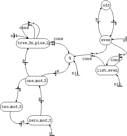
The resulting automaton, in file rinter.model.pl, is:
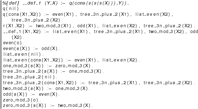
And graphically, this is the automaton of Figure 4.
Figure 4:
Lists starting with a number at least 3 as recognized in state
q of Figure
3
3.3.4 Converting Alternating to Non-Deterministic Tree Automata
All right, this starts being a tad intricate. In general, alternating
tree automata are not that easy to read. We may eliminate
intersection nodes ∧, and get a non-deterministic tree
automaton instead by using the -no-alternation option to h1. Either use
h1 -no-trim -no-alternation
instead of h1 -no-trim (this will produce a non-deterministic,
i.e., not an alternating tree automaton, in rinter.model.pl), or
simply run
h1 -no-trim -model
on rinter.model.pl to eliminate intersection nodes. Just as
h1 -no-trim
can be used to conv
ert an H1 clause set
into an equivalent alternating tree automaton,
h1 -no-trim -no-alternation
converts an H1 clause set, or an alternating tree
automaton, into an equivalent non-deterministic tree automaton. Run
pl2tptp rinter.model.pl >rinter_nd.p
h1 -no-trim -no-alternation rinter_nd.p
This yields the following automaton in file rinter_nd.model.pl.
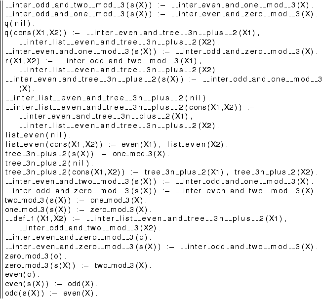
Using pl2gastex on the output
rinter_nd.model.pl, we arrive at the non-deterministic tree
automaton of Figure 5. This should be more
readable. The final state is q. Note that the result
still contains two copies of the automata recognizing respectively all
lists of even numbers, and all trees with leaves of the form nil or
3n+2, which are not needed any longer.
Figure 5:
Eliminating intersection nodes from Figure
4
The automaton of Figure 5, i.e., in file
rinter_nd.model.pl, uses new states such as
__inter_even_and_one__mod__3 (which recognizes all terms which
are both even numbers and numbers of the form 3n+1). In general,
these new states are named
__inter_P1_P2_…_Pn
and are meant to recognize all terms that are recognized
at P1 and at P2 and ... and at Pn at the same time. They
appear as P1 ∩ P2 ∩ … ∩ Pn under pl2gastex.
3.3.5 Purging Tree Automata
Well, Figure 5 should be more readable... but
there is some junk here. First, there are two sub-automata,
disconnected from the rest, defining the predicates zero_mod_3,
one_mod_3, two_mod_3, tree_3n_plus_2, and
odd, even, list_even. They do not contribute at
all to the definition of the language of r. Second, there are
also spurious states such as q, or __aux_1 (drawn as a
small state
 or
or
 ). Use plpurge to purge the automaton of
Figure 5 from all spurious states, by running
plpurge -final r rinter_nd.model.pl >rinter_nd.purged.pl
Figure 6:
Purging the automaton of Figure
5
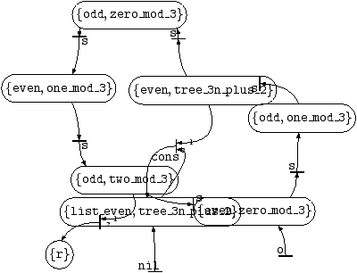
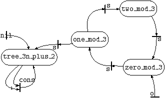
Hence we see that the relation r is simply the relation
relating all numbers that are both odd and equal to 2 modulo 3
(state odd ∩ two_mod_3) to all objects that are
both lists of even numbers and trees of with leaves equal to nil or
3n+2 (state list_even ∩ tree_3n_plus_2).
Looking a bit more in depth, the numbers that are both odd and equal
to 2 modulo 3 are 5, 11, 17, ..., in other words the numbers
that are equal to 5 modulo 6. And the objects that are both lists
of even numbers and trees of with leaves equal to nil or 3n+2 are
just lists of numbers equal to 2 modulo 6.
3.3.6 Determinizing Tree Automata
Looking at Figure 6, we realize that taking
the successor, i.e., applying the s function to a term
recognized at odd ∩ one_mod_3, yields a term that
is recognized both at even ∩ two_mod_3 and at
even ∩ tree_3n_plus_2. This is a form of non-determinism: we may want to travel to either state, not
knowing which will eventually lead to acceptance.
To cater for this, we may determinize our tree automata. This
produces an equivalent deterministic tree automaton, i.e., a set of
Horn clauses of the form
|
|
|
P (f (X1, …, Xn)) |
:- |
P1 (X1), …, Pn (Xn)
|
(5) |
|

By definition, a deterministic tree automaton can also be seen as a
partial function If from tuples of predicates to predicates, one
for each f. I.e., If (P1, …, Pn) = P if there is a,
necessarily unique, clause of the form (5).
To determinize the automaton rinter_nd.purged.pl of
Figure 6, run
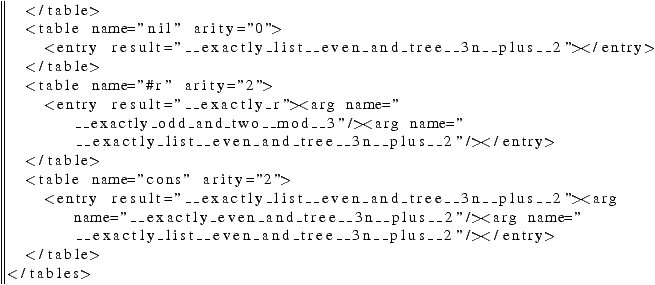
pldet rinter_nd.purged.pl >rinter_d.xml
This produces a deterministic tree automaton
in file rinter_d.xml:

The format will be explained in more detail in Section 7.
We can then convert this deterministic tree automaton into Prolog
notation, since every deterministic tree automaton is a particular
case of a non-deterministic tree automaton (itself a particular case
of an alternating tree automaton). Use auto2pl this way:
auto2pl rinter_d.xml >rinter_d.pl
This produces a file rinter\_d.pl, which is probably slightly
more readable than the XML file above:

Now draw the resulting automaton in Figure 7, using
pl2gastex:
pl2gastex rinter_d.pl >rinterd.tex
Figure 7:
Determinizing the automaton of Figure
6
The automaton of Figure 7 is not too big. But
beware: determinizing tree automata may produce automata that are
exponentially larger in the general case. In fact, pldet may
just take forever on some alternating, or even non-deterministic tree
automata.
3.3.7 Computing Unions, Transitive Closures
We have seen how to compute intersections of tree automata in
Section 3.3.2. Computing unions is just as easy.
Say that you want to compute the union of the sets of lists of even
numbers (listeven.p) and of the trees whose leaves are nil or
3n+2, n in |N. That is, instead of computing the intersection of
the languages L1 and L2 introduced at the
beginning of Section 3.3, we compute their union. As
before, build a file, say list_even_union_tree3plus2.p, by
concatenating the clauses from listeven.p and from
tree3plus2.p, but this time add the two clauses
| q (X) |
:- |
list_even (X) |
| q (X) |
:- |
tree_3n_plus_2 (X) |
list_even or by
tree_3n_plus_2. Concretely, run the
following commands:
OUT=list_even_union_tree3plus2
cat listeven.p tree3plus2.p >$OUT.p
echo "input_clause ("$OUT"_1, axiom, \
        [++q(X), --list_even(X)])." >>$OUT.p
echo "input_clause ("$OUT"_2, axiom, \
        [++q(X), --tree_3n_plus_2(X)])" >>$OUT.p
Now run h1 -no-trim as above:
h1 -no-trim list_even_union_tree3plus2.p
We get an equivalent
alternating tree automaton in the file
list_even_union_tree3plus2.model.pl:

Graphically, this is the alternating tree automaton of
Figure 8, again obtained using pl2gastex.
Figure 8:
Trees with leaves equal to
nil or to 3
n+2, or which are lists of even natural numbers
This can be determinized again. Run pldet and auto2pl :
pldet list_even_union_tree3plus2.model.pl \
  | auto2pl - >list_even_union_tree3plus2_d.pl
and you get

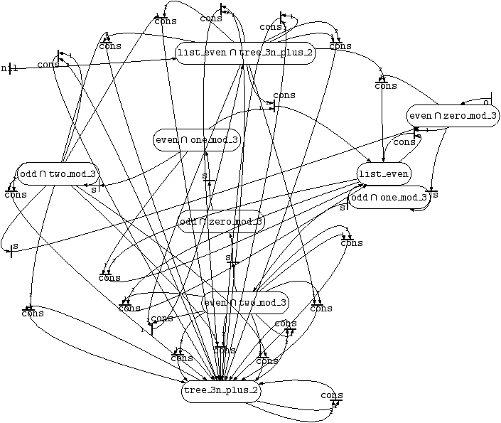
As you may see, the determinized automaton is much larger this time,
and pl2gastex now has real trouble trying to draw it. (See
Figure 9.) We use twopi as graph layout
engine here instead of neato and run:
pl2gastex -v -layout twopi \
  -overlap false \
  list_even_union_tree3plus2_d.pl \
   >list_even_union_tree3plus2_model_d.tex
Figure 9:
Determinizing the automaton of Figure
8
The trick we have used to compute intersections and unions, namely
concatenating files and adding new clauses (provided the concatenated
files agree on the semantics of predicates), can also be used to
compute other combinations of tree languages. A particularly
interesting one is the computation of transitive closures of
relations defined by tree automata (or, more generally, by H1 clause sets).
For the purpose of illustration, imagine you want to compute the
transitive closure of the binary relation r defined in
rinter_d.pl (drawn in Figure 7,
Section 3.3.6). Just create a fresh binary
predicate symbol r+, and add the clauses
| r+ (X, Y) |
:- |
r (X, Y) |
| r+ (X, Z) |
:- |
r (X, Y), r (Y, Z) |
OUT=rinter_d_plus
pl2tptp rinter_d.pl >$OUT.p
echo "input_clause (r_plus_r, axiom, \
        [++r_plus(X,Y), --r(X,Y)])." >>$OUT.p
echo "input_clause (r_plus_tc, axiom, \
        [++r_plus(X,Z), --r_plus(X,Y), --r_plus(Y,Z)])" >>$OUT.p
Compute an equivalent non-deterministic tree automata by
h1 -no-trim -no-alternation rinter_d_plus.p
You get

Since the clauses defining r+, i.e.,
r_plus, are the same as those defining r, the
transitive closure of r is r+ itself here:
r was already transitive. (Exercise: why?)
3.3.8 Complete Deterministic Tree Automata, Taking Complements
We observed in Section 3.3.6 that a deterministic
tree automaton could be seen as a partial function If from tuples
of predicates to predicates, one for each function symbol f.
A complete deterministic tree automaton is a set of Horn clauses of
the form (5), i.e.,
| P (f (X1, …, Xn)) |
:- |
P1 (X1), …, Pn (Xn) |
Any deterministic tree automaton can be completed to a complete one,
by adding a catch-all state __all (shown as ⊤ by pl2gastex), to which all missing transitions are directed. Precisely, if there
is an (n+1)-tuple (f, P1, …, Pn) such that there is not clause
as above, then add the clause
| __all (f (X1, …, Xn)) |
:- |
P1 (X1), …, Pn (Xn) |
The function If is then total. The collection of all such If
defines a finite model, whose set of values is that of all predicates.
A value satisfies a predicate P if and only if it is P, seen as a
value.
In fact, finite models and complete deterministic tree automata are
exactly the same notion. You might want to ponder this.
As an example, let us return to the Dreadsbury mansion murder mystery
(Section 3.2). As we have seen, the only to have
possibly killed Aunt Agatha is Aunt Agatha herself. We have proved
this by showing that the set of clauses in butler-puzzle.p (and
explained in Section 3.2) with WHO defined as
agatha was satisfiable.
Since this set is satisfiable, it has a model. Well, h1
computes such a model, in the guise of an alternating tree automaton.
Run
cpp -P -DWHO=agatha butler-puzzle.p >agatha.p
h1 -no-trim agatha.p
and you'll get it in file
agatha.model.pl (see Figure 10):

Figure 10:
Why Agatha killed herself
All right, this does not look like a model at all (much less an
explanation!), but remember there is a complete deterministic tree
automaton that is equivalent to it. We know how to compute an
equivalent deterministic tree automaton, using pldet and auto2pl, viz.
pldet agatha.model.pl | auto2pl - >agatha_d.pl
pl2gastex -v agatha_d.pl >agathad.tex
Using pl2gastex, as usual, produces a visual representation of it, see
Figure 11;
Figure 11:
Why Agatha killed herself, deterministically
So Agatha killed herself, Agatha is the only one not to be richer than
Agatha, Agatha hates herself and Charles, the butler hates Agatha and
Charles, and Charles hates noone.
Let us now produce the corresponding complete deterministic
tree automaton. This can be done using auto2pl, which we have already seen, using the -complete 1 option. Be warned, though, that complete deterministic tree automata
are large: with n states (included the catch-all states), any function taking k arguments will contribute nk clauses,
never less—and do not forget that any k-ary predicate symbol P
with k≥ 2 creates an invisible function symbol fP, which will
contribute nk clauses as well. Anyway, run
pldet agatha.model.pl | auto2pl -complete 1 - | sort >agatha_c.pl
and you'll get the resulting
complete deterministic tree automaton in file agatha_c.pl.
3.4 The Needham-Schroeder Symmetric Key Protocol Example
Try another example, nspriv.p, an encoding of the
Needham-Schroeder symmetric key protocol, together with three queries.
We do not mean that this is the only possible description of this
protocol, and only use this example as a motivation for using h1
with more complex clause sets.
Here are the clauses of nspriv.p, in Prolog notation. We have
shown the name of the clause on the left. First, we define a
predicate knows that is meant to recognize all messages that a
malevolent intruder is able to build. The first clauses say that
attackers can build any list of messages provided it knows each
message in the list, and conversely that it can build any message that
appears at any position in a list it knows:
|
|
intruder_knows_nil |
knows (nil) |
|
|
intruder_can_take_first_components |
knows (M1) |
:- |
knows (cons (M1, M2)) |
intruder_can_take_second_components |
knows (M2) |
:- |
knows (cons (M1, M2)) |
intruder_can_build_pairs |
knows (cons (M1, M2)) |
:- |
knows (M1), knows (M2) |
|
|
|
intruder_can_encrypt |
knows (crypt (M, K)) |
:- |
knows (M), knows (K) |
intruder_can_decrypt_if_has_private_key |
|
|
| |
knows (M) |
:- |
knows (crypt (M, key (pub, K))), |
| |
|
|
knows (key (prv, K)) |
intruder_can_decrypt_if_has_public_key |
|
|
| |
knows (M) |
:- |
knows (crypt (M, key (prv, K))), |
| |
|
|
knows (key (pub, K)) |
intruder_can_decrypt_if_has_symmetric_key |
|
|
| |
knows (M) |
:- |
knows (crypt (M, key (sym, X))), |
| |
|
|
knows (key (sym, X)) |
|
We also assume that there is an operation s that builds a new
message s (M) from an old M, in bijection with M; while we can
compute s (M) from M and recover M from s (M), the point is
that M and s (M) always differ.
|
|
intruder_can_compute_successors |
knows (s (M)) |
:- |
knows (M) |
intruder_can_compute_predecessors |
knows (M) |
:- |
knows (s (M)) |
|
In the Needham-Schroeder symmetric key protocol, Alice and Bob
communicate with a trusted server to get a common private key that
only they know, not the intruder. Alice can always start a session of
the protocol and send the server a triple containing Alice's identity
alice, Bob's identity bob, and a nonce, that is, a fresh message
for this session. Following [2001 (Blanchet)], we encode this
nonce as a function symbol applied to all parameters currently known,
say noncea (alice, bob)—the function symbol noncea
applied to Alice's identity alice and Bob's identity bob. Now we
assume a worst-case intruder model, where any communication can be
diverted by the intruder. The net effect is that, from a security
viewpoint, what Alice does by sending a message consists exactly in
making it known to the intruder:
|
|
alice_sends_message_1_to_server |
knows ( |
cons ( |
alice, |
| |
|
cons ( |
bob, |
| |
|
cons ( |
noncea (alice, bob), |
| |
|
|
nil)))) |
|
Just like sending a message consists exactly in making it known to the
intruder, receiving a message is modeled by stating that the intruder
was able to build this message. We shall therefore write a clause
saying that, if knows [A, B, Na] then knows crypt ([Na, B,
Kab, crypt ([Kab, A], Kbs)],
Kas). Note that we are effectively saying that, from
the angle of security, the actions of the server amount to adding new
capabilities to the intruder: if the intruder knows a message matching
what the server expects, it can build the message that the server will
answer, even though it may not know the long-term keys Kas and
Kbs.
Now we encode Kas as the term key (sym, cons (A, cons (server,
nil))), and Kbs as the term key (sym, cons (B, cons (server,
nil))); note that A and B are variables here, representing the
fact that the server will find these keys by looking up tables by the
identities of A, resp. B. In current sessions, we encode
Kab by the term key (sym, current_session (A, B, Na)). The
key Kab as generated during older sessions is encoded by the term
key (sym, old_session (A, B, Na)). Separating current from old
sessions means we have to write two clauses:
|
|
server_answers_A_with_encrypted_packet |
| |
knows (crypt ( |
cons ( |
Na, |
| |
|
cons ( |
B, |
| |
|
cons ( |
key (sym, current_session (A, B, Na)), |
| |
|
cons ( |
crypt (cons (key (sym, current_session (A, B, Na)), |
| |
|
|
cons (A, nil)), |
| |
|
|
key (sym, cons (B, cons (server, nil)))), |
| |
|
|
nil)))), |
| |
|
key ( |
sym, cons (A, cons (server, nil))))) |
| |
|
|
:- knows (cons (A, cons (B, cons (Na, nil)))) |
intruder_knows_previous_server_messages |
| |
knows (crypt ( |
cons ( |
Na, |
| |
|
cons ( |
B, |
| |
|
cons ( |
key (sym, old_session (A, B, Na)), |
| |
|
cons ( |
crypt (cons (key (sym, old_session (A, B, Na)), |
| |
|
|
cons (A, nil)), |
| |
|
|
key (sym, cons (B, cons (server, nil)))), |
| |
|
|
nil)))), |
| |
|
key ( |
sym, cons (A, cons (server, nil))))) |
| |
|
|
:- knows (cons (A, cons (B, cons (Na, nil)))) |
|
All right, now, when Alice receives the message from the server, she
should send the part encrypted with Kbs to Bob. The idea is that
while Alice can decrypt the whole message, which is encrypted with
Kas, only Bob can decrypt the sub-message that is encrypted with
Kbs. The message that Alice receives from the server should be
crypt ([Na, B, Kab, crypt ([Kab, A], Kbs)], Kas),
however she can only check that it is of the form crypt ([Na, B,
Kab, Msg) for some sub-messages Kab and Msg (which may be
totally unrelated to what the server actually sent). She can however
check that Na is the nonce noncea (alice, bob) that she created
earlier (see above, clause
alice_sends_message_1_to_server), and that
B really is Bob's identity bob. So Alice expects a message of the
form crypt ([noncea (alice, bob), bob,
Kab, Msg], Kas). As we
have said before, for Alice to receive this message, the intruder must
send it to Alice, so the intruder must be able to build it. Once
Alice receives this, it extract the sub-message Msg and forwards it
to Bob—in fact adding it to the set of messages known to the
intruder:
|
|
alice_gets_server_message_and_forwards_submessage_to_bob |
| |
knows (Msg) |
:-
knows (crypt ( |
cons (noncea (alice, bob), |
| |
|
|
cons (bob, |
| |
|
|
cons (Kab, |
| |
|
|
cons (Msg, nil)))), |
| |
|
|
key (sym, cons (alice, cons (server, nil))))) |
|
|
|
alice_gets_server_message_and_stores_current_session_key |
| |
alice_key (Kab) |
| |
|
:-
knows (crypt ( |
cons (noncea (alice, bob), |
| |
|
|
cons (bob, |
| |
|
|
cons (Kab, |
| |
|
|
cons (Msg, nil)))), |
| |
|
|
key (sym, cons (alice, cons (server, nil))))) |
|
Let's see what Bob does in this protocol. First, Bob expects to
receive the sub-message Msg above. Cutting it short, Bob decrypts
it, gets Kab, then sends a confirmation challenge crypt (Nb,
Kab), where Nb is a fresh nonce. As before, Nb is modeled
as a function symbol nonceb applied to all relevant variables.
|
|
agent_B_gets_forwarded_submessage_and_sends_confirmation_challenge |
| |
knows (crypt (nonceb (Kab, A, B), Kab) |
:- |
knows (crypt (cons (Kab, cons (A, nil)), |
| |
|
|
key (sym, cons (B, server, nil)))))) |
|
|
|
alice_answers_confirmation_challenge |
| |
knows (crypt (s (Nb), Kab)) |
:- |
alice_key (Kab), knows (crypt (Nb, Kab)) |
|
|
|
agent_B_checks_confirmation_from_A |
| |
bob_key (Kab) |
:- |
knows (crypt (s (nonceb (Kab, A, B)), Kab)) |
|
|
|
alice_is_an_agent |
agent (alice) |
|
|
bob_is_an_agent |
agent (bob) |
|
|
server_is_an_agent |
agent (server) |
|
|
intruder_is_an_agent |
agent (intruder) |
|
|
intruder_knows_all_agents |
knows (X) |
:- |
agent (X) |
|
|
|
intruder_knows_every_public_key |
knows (key (pub, X)) |
|
|
intruder_knows_own_private_key |
knows (key (prv, intruder)) |
|
|
intruder_knows_all_previous_session_keys |
knows (key (sym, old_session (A, B, Na))) |
|
|
Let us now ask a few queries. The first asks whether the intruder may
know the key Kab as it was generated by the server. The second
asks whether the intruder may know any key that Alice accepted as
being a key Kab at the end of the protocol. The third asks
whether the intruder may know any key that Bob accepted as being
Kab at the end of the protocol.
|
|
intruder_knows_session_key_generated_by_server |
| |
false |
:- |
knows (key (sym, current_session (alice, bob, Na))) |
intruder_knows_session_key_as_seen_by_alice |
| |
false |
:- |
alice_key (key (Mode, current_session (X, Y, N))), |
| |
|
|
knows (key (Mode, current_session (X, Y, N))) |
intruder_knows_session_key_as_seen_by_B |
| |
false |
:- |
knows (crypt (s (nonceb (Kab, A, B)), Kab)), knows (Kab) |
|
Now launch h1 on nspriv.p:
h1 nspriv.p
You should get
*** Derived: intruder_knows_session_key_as_seen_by_B ***
This means in short that h1 believes that this clause set is
unsatisfiable; in terms of protocols, that there is an attack. You
cannot actually be sure that this is indeed an attack, i.e., that this
clause set is indeed unsatisfiable, because this clause set is not in
the H1 format. (You should not conclude from this that
cryptographic protocols always produce clause sets outside H1, see [2002 (Nielson et al.)].)
In this case, and contrarily to the example of
Section 3.2, h1 computes an approximation of the input clause set S as a clause set S1,
and reasons on S1 instead. Check it using the -check-h1 2 option:
h1 -check-h1 2 nspriv.p
and you'll get the list of all clauses in nspriv.p that are not
in H1:
Warning: clause server_answers_A_with_encrypted_packet has
non-linear head, variable A occurs repeatedly.
Warning: clause intruder_knows_previous_server_messages has
non-linear head, variable A occurs repeatedly.
Warning: clause agent_B_gets_forwarded_submessage_and_\
\sends_confirmation_challenge
has non-linear head, variable Kab occurs repeatedly.
Warning: clause alice_answers_confirmation_challenge has two
non-sibling variables in the head that are connected
in the body, Nb and Kab.
Stop.
Note also that h1 gives you an explanation of what's going
wrong. For further explanation of what linear terms, sibling
variables and connected variables are, see [2002 (Nielson et al.)] or
[2005 (Goubault-Larrecq)].
The -check-h1 1 option runs the same checks. However, it still proceeds with checking
the (un)satisfiability of the approximated clause set S1, even when
the approximation is not exact, i.e., when the original clause set S
is not in H1.
The approximated clause set S1 is always in the class H1, and always implies S logically. In particular, if h1
does not find any contradiction, i.e., if S1 is satisfiable, then
S is satisfiable, too. In terms of cryptographic protocols, if h1 tells you that your protocol has no attack, then you can be sure
of it. (That is, up to the accuracy of your model, written as
clauses.)
In our case, h1 found a purported attack, i.e., a purported
contradiction. It turns out that nspriv.p is indeed
contradictory. In fact, in most cases where h1 thinks a clause
set is contradictory, it is indeed contradictory. (Although, as
usual, your mileage may vary.)
We terminate this example by mentioning the -all option.
The answer
*** Derived: intruder_knows_session_key_as_seen_by_B ***
above means that h1 found a (purported) contradiction first, and
second that, in order to derive the empty clause false, h1
required the clause
intruder_knows_session_key_as_seen_by_B.
Is this the only query that fails? Remember we have asked three
queries. One way of checking this is to remove the
intruder_knows_session_key_as_seen_by_B
clause from nspriv.p and run h1 again. There is a simpler
option: run h1 with the -all option. Once a contradiction has been found, instead of stopping just
like any other prover, h1 -all will continue, trying to find
contradictions using other queries.
On the example, running
h1 -all nspriv.p
you will get the same answer as above:
*** Derived: intruder_knows_session_key_as_seen_by_B ***
In other words, no other query fails. In terms of security, this
means that while Bob's key Kab is not secure, those of Alice and
the server definitely are. This may seem paradoxical, however the
attack that h1 just found is one where the intruder deceives Bob
into accepted an old, cracked key from an older session. This key is
not the key that the server produced. It is also old, meaning that it
will be detected as not being new by Alice's use of the nonce Na.
We have just proved that Alice and the server were in fact safe in
this protocol, while Bob is not.
The -no-resolve option can be used to disable the reasoning facilities of h1
altogether. Then h1 -no-resolve will just compute an
approximation of the input clause set, and store it into the log file.
For example,
h1 -no-resolve nspriv.p
runs without any output, and creates the log file nspriv.log.gz.
As we have already said, it is not really instructive to look at this
file directly.
However, you can extract from it the approximated clause set by
running:
h1getlog processed nspriv.log | pl2tptp -
This will output the approximated clause set on stdout: h1getlog with the processed option will extract the
approximate clauses and print them in Prolog format. Then pl2tptp with the - argument (meaning stdin) will convert
these from Prolog format to TPTP format.
All this can be done in a simpler way, by using the -log-out option to h1. Then h1 will output its log file
to stdout. You can then pipe it to h1getlog and pl2tptp, as follows.
h1 -log-out -no-resolve nspriv.p | h1getlog processed | pl2tptp -




 or
or
 ). Use plpurge to purge the automaton of
Figure 5 from all spurious states, by running


